Estimating causal policyFX with clusteredinterference
Brian G. Barkley
2019-03-17
Source:vignettes/estimate-policyFX.Rmd
estimate-policyFX.RmdFirst, load the clusteredinterference package
library(clusteredinterference)Now load a quick data example that’s included in the package
data("toy_data") Estimation
Estimation is implemented with the policyFX() function:
suppressWarnings(RNGversion("3.5.0")) ## For backwards compatibility
set.seed(1113)
causal_fx <- policyFX(
  data = toy_data,
  formula = Outcome | Treatment ~ Age + Distance + (1 | Cluster_ID) | Cluster_ID,
  alphas = c(.3, .5),
  k_samps = 1
)
The policyFX() function outputs a "policyFX" object, which works well with a few methods, including:
summary(causal_fx)
#> ------------- causal estimates --------------
#>     estimand estimate     se     LCI    UCI
#>      mu(0.3)   0.6523 0.0635  0.5279 0.7767
#>      mu(0.5)   0.6075 0.0505  0.5086 0.7063
#>     mu0(0.3)   0.6707 0.0736  0.5264 0.8151
#>     mu0(0.5)   0.5849 0.0728  0.4422 0.7276
#>     mu1(0.3)   0.2799 0.0563  0.1695 0.3902
#>     mu1(0.5)   0.3974 0.0577  0.2842 0.5105
#>  OE(0.5,0.3)  -0.0449 0.0366 -0.1165 0.0268
#>  OE(0.3,0.5)   0.0449 0.0366 -0.0268 0.1165
#>
#>           ... and 4 more rows ...
#>
#> -------------- treatment model -------------
#> Generalized linear mixed model fit by maximum likelihood (Adaptive
#>   Gauss-Hermite Quadrature, nAGQ = 2) [glmerMod]
#>  Family: binomial  ( logit )
#> Formula: Treatment ~ Age + Distance + (1 | Cluster_ID)
#>    Data: data
#>      AIC      BIC   logLik deviance df.resid
#> 137.0345 147.3743 -64.5172 129.0345       94
#> Random effects:
#>  Groups     Name        Std.Dev.
#>  Cluster_ID (Intercept) 1.18
#> Number of obs: 98, groups:  Cluster_ID, 30
#> Fixed Effects:
#> (Intercept)          Age     Distance
#>    -1.44609     -0.00851      0.26097
#>
#> ------------- propensity scores -------------
#>      1      2      3      4      5      6      7      8      9     10
#>  0.105  0.162  0.086  0.102  0.167  0.045  0.244 0.0934 0.0765  0.197
#>     11     12     13     14     15     16     17     18     19     20
#> 0.0653  0.281  0.104  0.365 0.0867  0.198  0.207  0.106 0.0847  0.134
#>     21     22     23     24     25     26     27     28     29     30
#>  0.103  0.111  0.105  0.302 0.0434 0.0943 0.0443 0.0512   0.13  0.263
#> ---------------------------------------------
Necessary arguments
data
A data.frame. At present, tibbles are coerced back to standard data.frames. I also recommend against using factors in the columns.
alphas
A numeric vector of probabilities corresponding the the policies of interest. Each must be between 0 and 1.
k_samps
The user must specify the number of sum-sampled vectors for estimating the counterfactual probabilities (nuisance parameters). It is recommended to choose k_samps <=5. To avoid the sub-sampling approximation and use all possible vectors, set k_samps=0.
formula
The formula may be the trickiest, and it has plenty of information. It provides:
outcome | treatment ~ predictors and random intercept | clustering specificationNote that the middle section is passed to glmer() to fit the mixed effects model, so this is how to specify the modeling formula.
Treatment ~ Age + Distance + (1 | Cluster_ID)See below for the model output.
Formal arguments with defaults
root_options = NULL
This is for rootSolve::multiroot() used in the point estimation procedure. E.g., this will be passed in:
root_options = list(atol = 1e-7)
nAGQ=2
This is for lme4::glmer(). The default in glmer() is nAGQ=1, which indicates a Laplace approximation to the log-likelihood. Instead, in this package the default is nAGQ=2, which indicates that n=2 Adaptive Gaussian Quadrature points will be used. This is slightly slower but is a more accurate calculation. In limited testing, it seems that nAGQ=2 was almost as accurate as higher values, so 2 was chosen as the default. See their documentation for more details.
Dots tricks
In the event you’re only interested in a subset of contrasts, you can pass a customized grid into the function.
my_grid <- makeTargetGrid(alphas = (3:8)/20, small_grid = TRUE)
head(my_grid)
#>   alpha1_num alpha2_num trt alpha1 alpha2 estimand effect_type estVar
#> 1          1         NA  NA   0.15     NA       mu     outcome   TRUE
#> 2          2         NA  NA   0.20     NA       mu     outcome   TRUE
#> 3          3         NA  NA   0.25     NA       mu     outcome   TRUE
#> 4          4         NA  NA   0.30     NA       mu     outcome   TRUE
#> 5          5         NA  NA   0.35     NA       mu     outcome   TRUE
#> 6          6         NA  NA   0.40     NA       mu     outcome   TRUE
This can be particularly useful for plotting, as you can “turn off” the variance estimates
my_grid$estVar <- FALSEThis is available through the dots argument. Note that when supplying a custom target_grid, it’s not necessary to specify the alphas argument, as that is taken directly from target_grid.
causal_fx2 <- policyFX(
  data = toy_data,
  formula = Outcome | Treatment ~ Age + Distance + (1 | Cluster_ID) | Cluster_ID,
  # alphas = c(.3, .5),
  target_grid = my_grid,
  k_samps = 5,
  verbose = FALSE,
  root_options = list(atol=1e-4)
)

print(causal_fx, nrows = 9)
#> ------------- causal estimates --------------
#>      estimand estimate     se     LCI      UCI
#>       mu(0.3)   0.6523 0.0635  0.5279  0.77667
#>       mu(0.5)   0.6075 0.0505  0.5086  0.70633
#>      mu0(0.3)   0.6707 0.0736  0.5264  0.81506
#>      mu0(0.5)   0.5849 0.0728  0.4422  0.72760
#>      mu1(0.3)   0.2799 0.0563  0.1695  0.39020
#>      mu1(0.5)   0.3974 0.0577  0.2842  0.51055
#>   OE(0.5,0.3)  -0.0449 0.0366 -0.1165  0.02681
#>   OE(0.3,0.5)   0.0449 0.0366 -0.0268  0.11651
#>  SE0(0.5,0.3)  -0.0858 0.0403 -0.1648 -0.00677
#>           ... and 3 more rows ...
#> ---------------------------------------------
Plotting
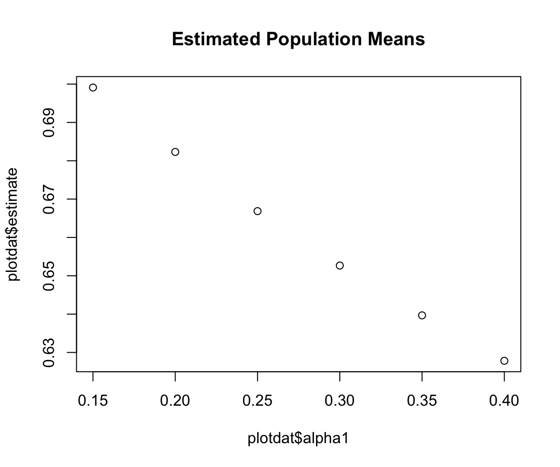
The tidy dataframe estimates can be easily used for plotting:
plotdat <- causal_fx2$estimates[causal_fx2$estimates$estimand_type=="mu",]
plot(x = plotdat$alpha1, y = plotdat$estimate, main = "Estimated Population Means")
Treatment model
As mentioned above, the treatment model is specified via the formula argument. For example, compare:
# Returns the specified formula, coerced to a Formula object
causal_fx$formula
#> Outcome | Treatment ~ Age + Distance + (1 | Cluster_ID) | Cluster_ID
# causal_fx$model is a glmerMod S4 object
causal_fx$model@call
#> lme4::glmer(formula = Treatment ~ Age + Distance + (1 | Cluster_ID),
#>     data = data, family = stats::binomial, nAGQ = nAGQ)
lme4::getME(causal_fx$model, c("beta", "theta"))
#> $beta
#> [1] -1.446087049 -0.008509771  0.260968952
#>
#> $theta
#> Cluster_ID.(Intercept)
#>               1.180325